
Abstract
In September of 2023, ZKM Research started developing a zkVM for the MIPS instruction set and processor architecture. This paper presents a high-level description of the system and software architecture, including the rationale for the most important design decisions. zkMIPS is available in github.com/zkMIPS/zkm and more about ZKM can be found in zkm.io.
A zkVM is a primitive which permits one party A to outsource a computation to another (computationally more powerful) party B in a verifiable manner. The output computed by B comes with a proof (or seal) that the result was computed correctly. In the case of zkMIPS, the program to be executed is specified using a subset of MIPS instruction set, possibly after compilation from some other language.
A valid computation can be interpreted as a sequence of valid states, which can be compiled to a table whose columns represent CPU variables and rows represent steps of the computation process. This table is known as the trace record (or trace). Moving from one row of the trace to the next represents a state transition, which must correspond to a valid computation step. In this setup, verifying the correctness of a computation is equivalent to verifying the transition between each pair of subsequent rows of the trace record. One way to make this verification more efficient is to encode the entire trace record as a mathematical object, usually a polynomial, in a process called arithmetization.
Another important building block for zkVMs is the routine run between A and B to help the verification of the desired polynomial properties. The polynomial resulting from the arithmetization process is usually of the size (degree) of the program being proved, meaning verifying this polynomial naively has roughly the same complexity of verifying the program itself. To optimize this process, the parties involved engage in several rounds of a challenge-response game where B sends some commitment data to A, A makes a challenge to B, and B responds to it. Using the data provided by B beforehand and the responses to their queries, A can convince themself that B did not cheat along the way.
The range of IOPs used for succinct verification is somewhat small, but the range of arithmetiza tion techniques is large and choosing among them is not easy. In the first place, the mathematical theories involved are highly abstract, not easy to comprehend, and often there is no consensus terminology among works in the area. This is aggravated by the fact that what is described in a paper is not necessarily what has been implemented, while these digressions often are not well-documented. One either has access to high-level theoretical papers or low-level access to existing open-source libraries that contain very little documentation on an intermediate level. Of course, these low-level libraries are highly relevant in order to reduce development time while obtaining good performance.
The main purpose of this paper is to describe this confusing landscape in detail, and discuss the choices made by the zkMIPS team. This document covers the theoretical aspects of the arithmetization models and IOPs used in zkMIPS, as well as the design choices made during the development process. Where theory and practice do not align, we opted to privilege the way the protocol is implemented and often ignore details that are better explained in the original papers. In other words, this work aims to enlighten developers by plugging the gap between papers and code. We provide this kind of information as guidance and we believe that it will be intrinsically useful for the community, independent of zkMIPS.
The past 2-3 years have seen the rise of numerous projects with similar objectives to zkMIPS’s. zkEVMs such as zkSync[15], Scroll[25], Polygon Miden[19] and Taiko[28], implement verifiable computing for Ethereum’s EVM bytecode, while zkVMs such as Zilch[7], o1VM[17], RISC0[22], Jolt[3], SP1[27] and Valida[29] implement verifiable computing for off-chain instruction set architecture (ISA). Some zkVMs define their own ISA, while others are based on real-world ISAs such as MIPS[16] and RISC-V[21].
We chose MIPS over RISC for a variety of reasons. First, it is open-source and has been around for 40 years with a strong presence in industry. Almost any language can compile to some variation of the MIPS ISA, making the range of MIPS applications go from legacy to IoT. The MIPS-R3000[11] variation, in particular, has not changed over time and is considered one of the most reliable ISAs, unlike EVM bytecode (have frequent minor opcode changes) or RISC-V (allows custom instructions). As a result of this popularity and stability one could say anything compiles to MIPS and MIPS compiles to anything, which give us a reasonable advantage over zkVMs based on other architectures.
Zilch[7] and o1VM[17] are the only other MIPS-based zkVMs we are aware of (most of the other zkVMs are LLVM or RISC-based). Zilch has been around since before zkMIPS development and it was used as a study-case for our design. It was written with the libSTARK[13] library, making it fully STARK-based, and restricts itself to a MIPS subset called zMIPS. Besides the VM, Zilch defines a variation of Java programming language called ZeroJava, and implements a ZeroJava to zMIPS compiler. O1VM, on the other hand, is more recent and based on good zkVM practices established after Zilch.
Section 2 describes the MIPS architecture as specified by zkMIPS codebase, which includes certain assumptions for the sake of simplification. Section 3 gives a general description of arguments-of knowledge, specially SNARK and STARK, which might serve as an introduction to ZK for those not familiar with the concept of cryptographic proofs. The content of the previous two sections come together in a description of the zkMIPS proving architecture given in Section 4. Finally, Section 5 discusses the performance of the current zkMIPS implementation.
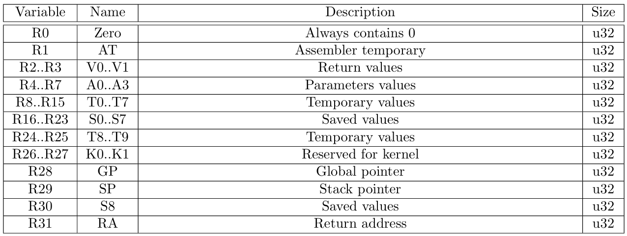
The Microprocessor without Interlocked Pipelined Stages (MIPS) is a well-known and widely adopted class of 32/64-bit computer architectures developed by MIPS Computer Systems. The 32-bit specification is a big-endian, register-based architecture with 32 general purpose registers (GPRs) of 32-bit each, allocated according to Table 1, and a 4GB memory addressed by 232 words of 4 bytes each.
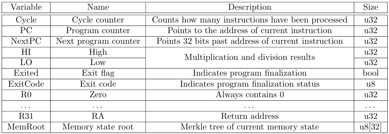
In general, MIPS programs operate on a 32-bit cycle counter, a 32-bit program counter representing the memory address of the current instruction (optionally, the next value of this counter might be stored in a separate register), 32-bit high and low results for 32-bit multiplication and division operations, an exit boolean, and an 8-bit exit flag. In addition to these, zkMIPS also operates over a 32-bit representation of the memory state defined as the Poseidon-based[14] Merkle root whose leaves correspond to 4KB memory pages. A list of all variables contained in zkMIPS state is given in Table 2.
This memory state representation is necessary to track changes in the memory and guarantee memory consistency during the execution of the VM. Furthermore, all variables included in intermediary states of the MIPS VM (i.e. counters, high/low results, and exit variables) are recorded in memory after each cycle. This approach allows steps of the execution of this VM to be described more easily because only those CPU states variables that have changed in a given transition are recorded in memory, while those that have not changed will have their consistency ensured by memory constraints.
The constraints that ensure memory consistency are created in parallel to changes in CPU states. This approach is possible because even though these constraints model changes in the memory space modified by the VM, their consistency depends only on the hash used to compute the Merkle tree. How this and several other parallel procedures run in zkMIPS will be explained in Section 4. In Section 2.1 we delimit and describe the subset of MIPS instructions supported by zkMIPS CPU.
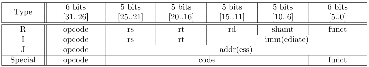
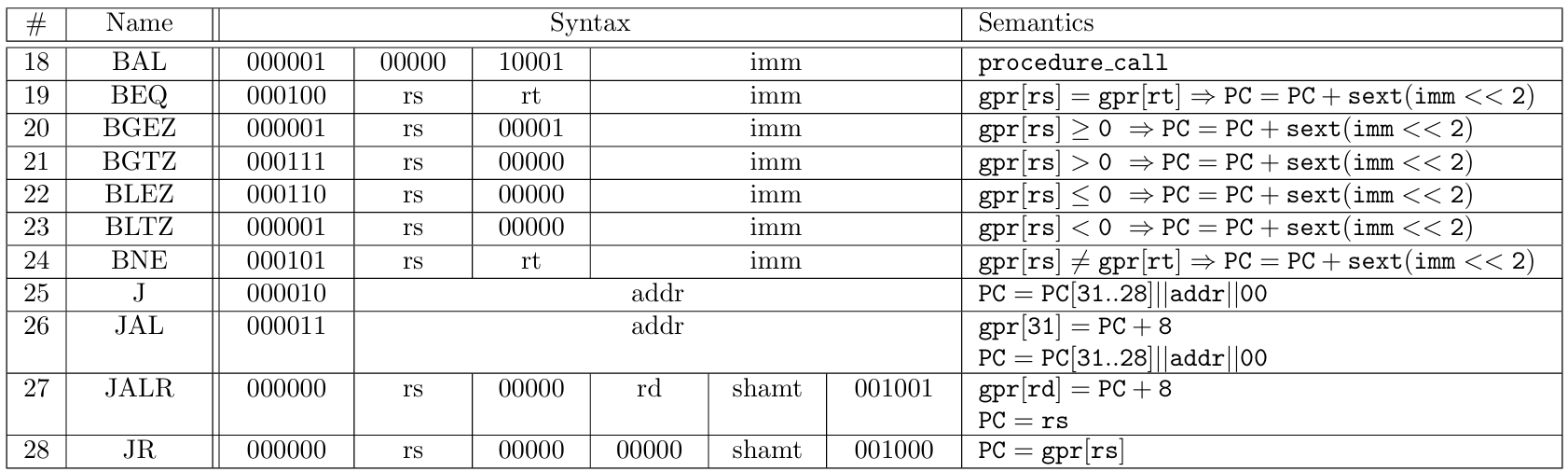
zkMIPS supports a subset of 71 MIPS instructions of 32 bits each. The first or the last 6 bits of an instruction are used for identification. The first 6 bits of an instruction are called the opcode and, when an instruction has opcode 000000, its last 6 bits are called funct. The values contained in the opcode and funct fields define the syntax and the semantics of each instruction. MIPS instructions have four possible syntax formats, namely the R, I, J and special-formats. Instructions that have functs are usually of the R or the Special-formats, and instructions that do not are of the I or the J-formats.
The 20 bits between opcode and funct of R-format instructions are divided into four 5-bit fields, with the first two encoding input registers, the third encoding an output register, and the last encoding an extra input for some instructions. The last 26 bits of I-format instructions are divided into two 5-bit fields encoding two inputs or one input and one output registers, and one 16-bit field encoding a half-word input. The last 26 bits of J-format instructions encode one single input. There is also one special-format for instructions that invoke system events, this one with the last 6 bits encoding a funct field and the middle 20 bits encoding one single input. This scheme is illustrated in Table 3.
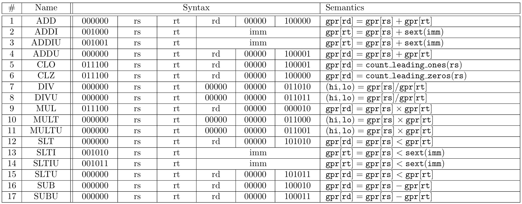
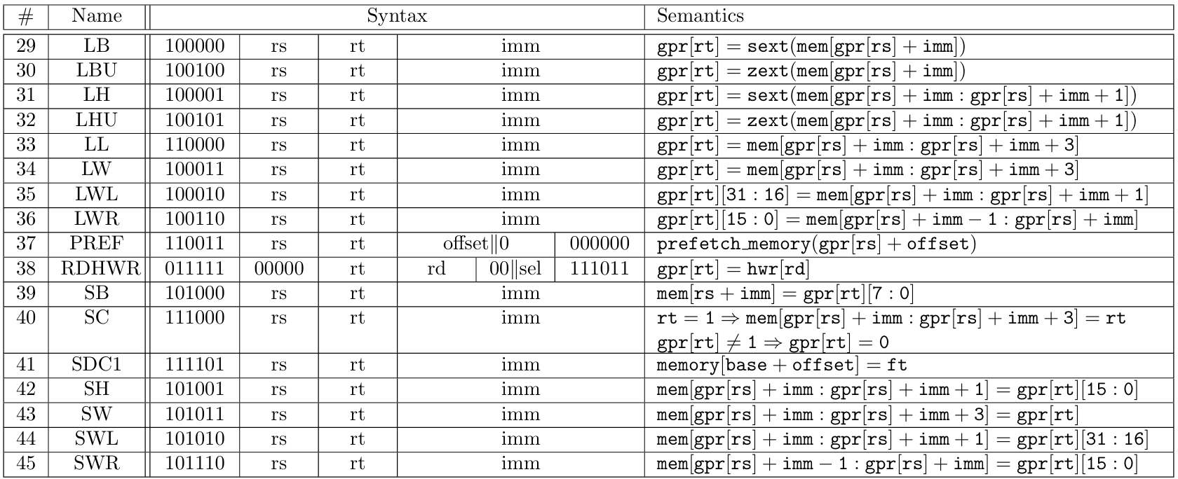
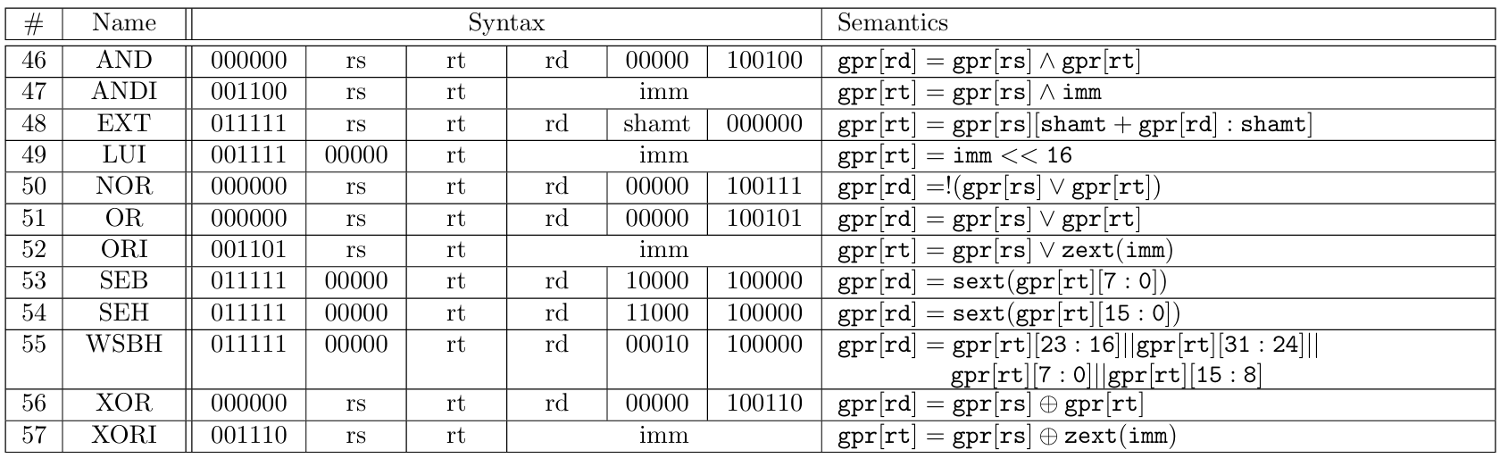
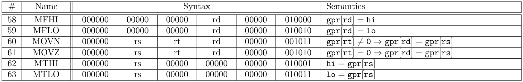
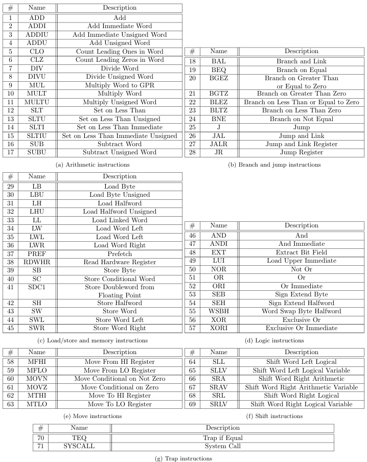
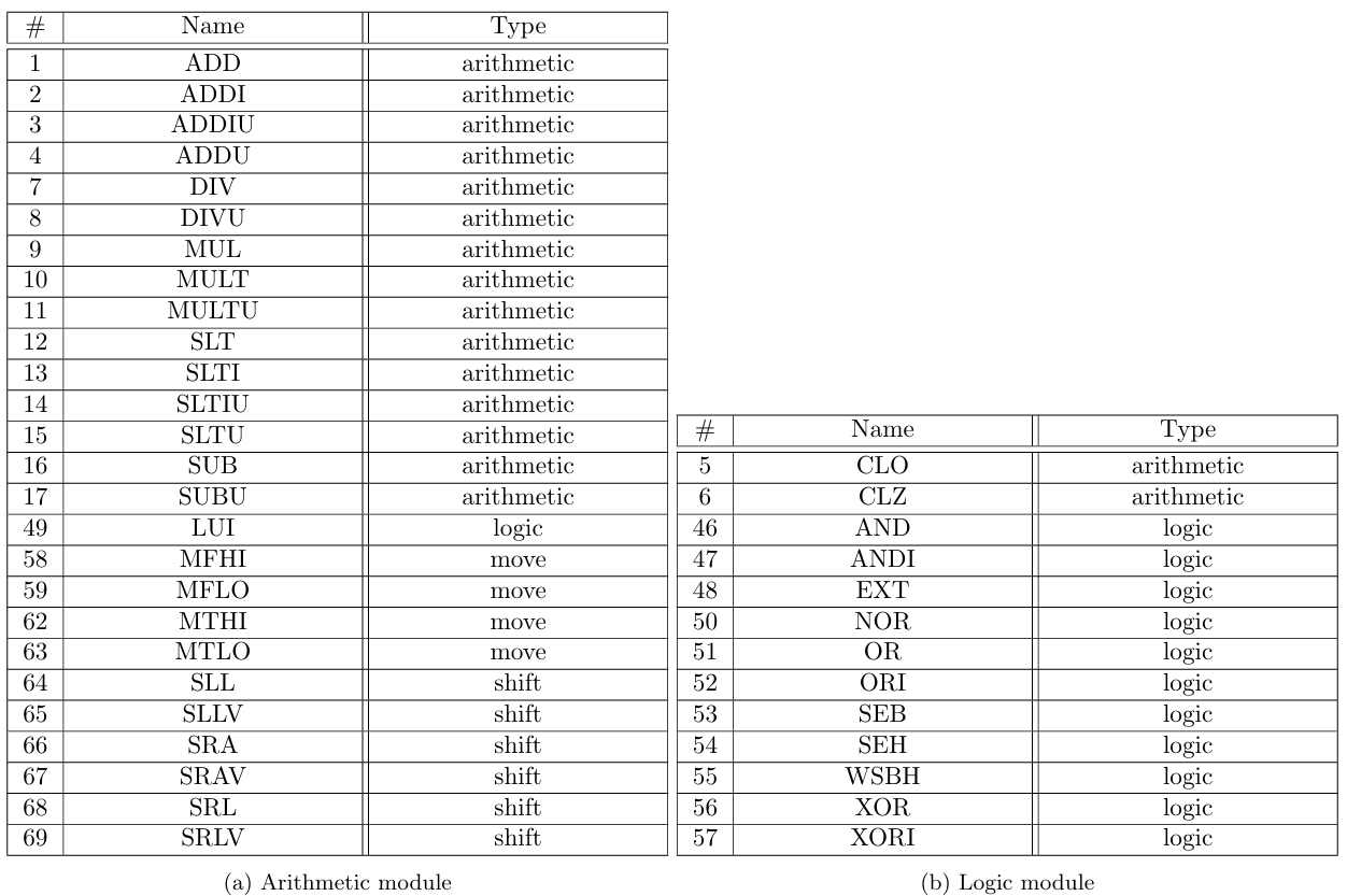
The 71 MIPS instructions supported by zkMIPS belong to 7 original MIPS instruction categories, namely arithmetic, branch and jump, load/store and memory, logic, move, shift and trap, as described in Tables 4 to 10 and listed in Table 11. These categories relate to how instructions are modeled in zkMIPS, as explained in Section 4.3.
Instructions from the arithmetic category perform arithmetic operations over 32-bit values stored in input registers (R-format instructions) or signed 16-bit inputs (I-format instructions). These 16-bit inputs are extended to 32-bit inputs according to their sign (the sext function from Table 4 represents
a signed extension). The same happens for signed 16-bit inputs from branch and jump instructions and for some from load/store and memory instructions (see Tables 5 and 6, respectively). Unsigned 16-bit inputs from remaining load/store and memory instructions are handled differently; they can be simply extended with zeros (the zext function from Table 6 represents a zero extension).
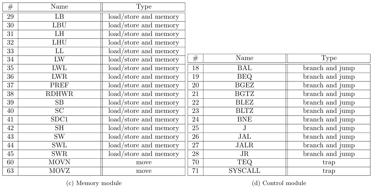
Instructions from the branch and jump category modify the PC according to signed 16-bit inputs (I-format branch instructions), unsigned 26-bit inputs (J-format jump instructions) or 32-bit values stored in registers (R-format jump instructions). Signed 16-bit inputs correspond to instruction indexes relative to the current PC, while unsigned 26-bit inputs and 32-bit values stored in registers correspond to absolute instruction indexes. Since memory is byte-aligned and the PC corresponds to the address of the current instruction, instruction indexes must be converted to the instruction addresses. To do so, signed 16-bit instruction indexes are shifted 2 bits to the left, then extended and added to PC so they can address memory positions within the 217 bytes (128kB) memory range from the current PC. Analogously, unsigned 26-bit instruction indexes are padded with 2 zeros to encode byte-aligned addresses instead of word-aligned, and then appended to the first 6 bytes from PC so they can address memory positions within the 218 bytes (256MB) memory region the current PC points to.
Instructions from the load/store category perform memory operations based on input or output registers, base memory positions stored in registers and 16-bit memory offsets (I-format instructions). Values loaded from memory can be signed or zero extended, depending on the opcode. The memory position from which bytes, half-words or words are loaded is given as an unrestricted byte index, meaning they can be loaded from byte indexes inside memory words (one can load the byte sequence [0x06,0x09] as a word even though it intersects different memory words, [0x04,0x07] and [0x08,0x0a]). In addition to that, left or right halves of registers can be loaded or stored while maintaining the other half unchanged, and there are instructions to lock memory position atomically. For a better comprehension on how load/store and memory instructions are defined, we refer to MIPS Manual[16].
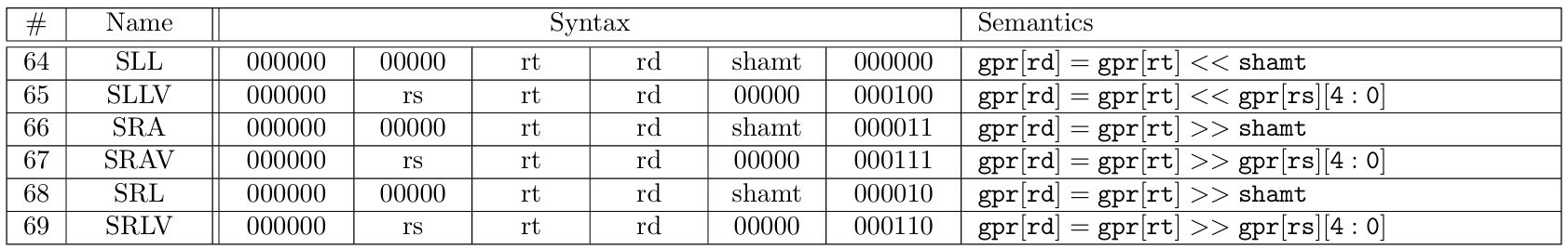
Instructions from the logic category perform usual logic operations over 32-bit values stored in input registers (R-format instructions) or 16-bit inputs (I-format instructions). In addition to these operations, the logic category also features an instruction to load 16-bit inputs (I-format instructions) to the upper-most half of a GPR. Instructions from the move category copy 32-bit values between GPRs (R-format instructions), or between general-purpose and high/low registers. Instructions from the shift category perform arithmetic or logical shifts over GPRs, according to 5-bit values stored in input registers or shamt fields (R-format instructions). Finally, instructions from the trap category invokes special kernel functions according to 32-bit values stored in input registers (R-format instructions) or 20-bit inputs (special-format instructions). For details we refer to [16].

Cryptographic proof systems (or just proof system) can model algorithms as 2-party protocols in contexts where one of the parties can run the underlying algorithm faster (B from Section 1) than the other (A). Usually, the privileged party either has access to a more efficient computer or possesses some secret information, and the resulting protocol allows this party to convince the other one that the underlying algorithm can be executed correctly when run on an efficient computer or when fed with secret information. For this reason, we denominate the convincing party the Prover, the convinced party the Verifier, and the 2-party protocol they engage in a cryptographic proof (or just proof ).
Proof systems should be designed to optimize the interests of both the Prover and the Verifier. On the Prover side, this means the proof succeeds (the Verifier is convinced) with high probability when the Prover is faithfully following the protocol, i.e. it can execute the underlying algorithm successfully and follows the protocol description correctly. This property is called completeness. On the Verifier side, the proof system should guarantee the proof succeeds with negligible probability when the Prover is maliciously engaged in the protocol, i.e. it cannot execute the underlying algorithm successfully or it does not follow the protocol description. This property is called soundness.
To enable particular proof designs, the soundness of some proof systems may be restricted to polynomial-time Provers, in which case we call the resulting protocol a cryptographic argument (or just argument). Additionally, some proof systems may guarantee with high probability that the Prover knows some information that allows it to run the underlying algorithm, in which case we call the resulting protocol a proof-of-knowledge. When a proof system produces a protocol with these two properties (it guarantees with high probability that a polynomial-time Prover knows some information that allows it to run the underlying algorithm), we call the resulting protocol an argument of knowledge. Since proofs and arguments are similar, we might use proof when referring to both.
The communication between Prover and Verifier, which includes public parameters and messages exchanged during the protocol execution, is called the transcript. Formally, for a proof to be considered a proof-of-knowledge, there must exist an algorithm called Extractor that recovers the secret information when given access to transcripts from equivalent but different instances of the same proof. When a proof-of-knowledge keeps any secret information secure, we call it Zero-Knowledge (ZK). Formally, for a protocol to be considered ZK, there must exist an algorithm called Simulator that produces a fake transcript in a way to make it statistically indistinguishable from a real one.
Modern proofs are often required to run in time polynomial in the logarithm of the input to the underlying algorithm. In other words, as this input size N increases, Prover and Verifier execution times increase polynomially on log (N). When communication complexity is also polynomial on log (N), we say the proof is succinct. Even though the ZK in zkVM means Zero-Knowledge, we stress that these proofs are often only required to be succinct, meaning a protocol might not be private and still be considered a zkVM because it is succinct. Modern proofs are also often required to be non-interactive, meaning the Verifier can be convinced without direct interaction with the Prover. In this case, we use the term proof to refer to the data produced by the Prover to indirectly convince the Verifier.
Non-interaction is useful when applying cryptographic proofs to distributed systems because it allows one single Prover to convince multiple Verifiers with the same proof. Assuming non-random values sent by the Verifier during an interactive proof can be deterministically computed by the Prover, it can be made non-interactive by replacing random values chosen by Verifier with verifiable random values chosen by the Prover, such as hash function outputs carefully queried using partial transcripts. This technique, known as Fiat-Shamir transformation[1], can be applied to most interactive proofs.
The advent of blockchain technologies encouraged the development of succinct and non-interactive arguments-of-knowledge, usually abbreviated to SNARKs. Originally, this term referred to a specific proof system[23], but gradually began to refer to a range of proof systems targeting blockchain-related verification whose properties often rely on some well-formatted public and random input called Common Reference String (CRS). The procedure to format this random input depends on the proof system and is defined accordingly by means of an accompanied algorithm called Generator.
The need for running a Generator before the Prover makes it difficult to apply some proof systems to the blockchain context, since the main principle of blockchain is decentralization. In practice, the risk of a centralized Generator to cheat is mitigated by running an equivalent secure multi-party computation, meaning the Generator is reformulated as a distributed protocol that produces the same output. The main challenge here is to prove the correct execution of this protocol, which is still a source of criticism to early blockchain projects that adopted SNARKs[31]. Furthermore, this protocol might need to be re-executed if the complexity of the statements that must be proven increases, since the CRS produced by a Generator is capable of proving algorithms up to a certain number of steps.
In this context, new proof systems tried to address the requirements from this new age of cryptographic proving applications. These proof systems are scalable and transparent (non-interactive) arguments-of-knowledge, usually abbreviated to STARKs. As was the case for SNARKs, this term referred to a specific proof system[8], but gradually began to refer to a range of similar proof systems. The choice to privilege scalability and transparency over succinctness means proofs might be larger and take longer to produce, but do not rely on a Generator. Instead, they rely on reasonable cryptographic assumptions (transparency) and can be generated despite the algorithmic complexity (scalability).
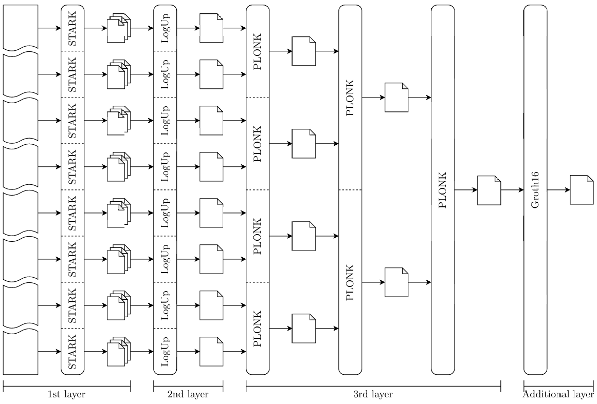
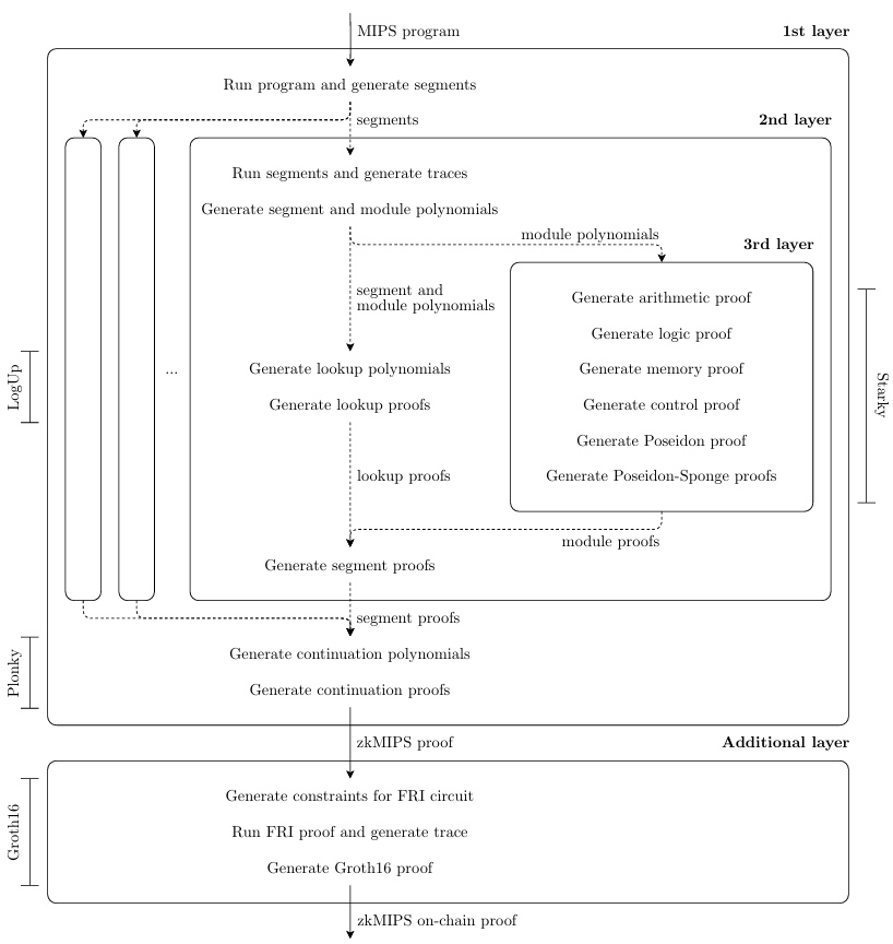
zkMIPS employs variations of the STARK[8] and PLONK[4] (SNARK) proof systems, as well as Groth16[12] (SNARK) and the latest version of the LogUp[26] protocol. STARK, PLONK and Groth16 are general-purpose arguments-of-knowledge, whereas LogUp is an argument for the correspondence between two public vectors (in the actual proving procedure, LogUp is used to combine smaller STARK proofs). The zkMIPS proving procedure is recursive and divided into four layers, as illustrated in Figure 1. STARK, LogUp and PLONK generate proofs in the first three layers, in that order, whereas Groth16 is used to generate proofs in an optional layer whenever the final proof must be verified on-chain.
Mandatory proofs are written[32] using the Plonky2[20] framework, which implements in Rust variations of the STARK and PLONK proof systems (the LogUp from the second layer is implemented as a STARK proof). In other words, we use this library to write the Prover, compile it using a Rust compiler, and produce the actual proofs passing a MIPS program as input to the compiled Prover.
These proofs can be verified with a program written in Rust using the same library. Optional proofs are written[33] using the GNARK[6] library, and can be verified with a smart-contract written in Solidity.
The STARK and PLONK variations implemented by Plonky2 are called Starky and Plonky, respectively. The Starky borrows pieces from PLONK and the Plonky borrows pieces from STARK. The pieces Plonky borrows from STARK make it transparent, which might induce some people to consider it a STARK, but the pieces Starky borrows from PLONK do not make it more succinct. Because the difference between SNARK and STARK is tenuous but might interest most readers, Section 3.1 explains modern SNARKs and STARKs design, and what differs them in practice. Section 3.2 explains the differences between PLONK, STARK and their Plonky2 counterparts.
To prove an algorithm, general-purpose cryptographic proof systems (as STARK, PLONK and Groth16) require a public input that expresses that algorithm as a finite automaton. Early SNARKs[23, 12] represented algorithms as Quadratic Arithmetic Programs (QAP), meaning steps of the algorithm should be input to the proof as a system of constraints where each constraint represents a product of two linear combinations that result in a third linear combination, as in Equation 1.

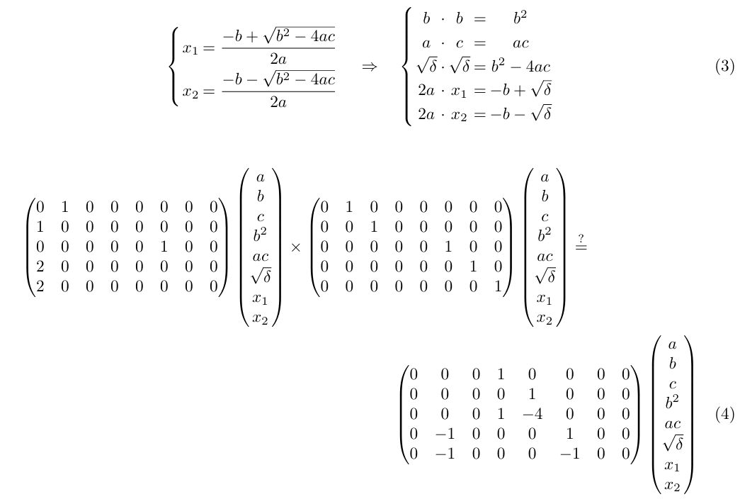
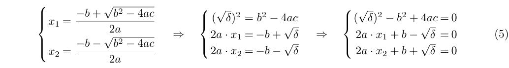
The intuition behind QAP is that linear combinations can be obtained by multiplying a matrix and a vector, allowing Equation 1 to be compiled into Equation 2, where A, B and C are public matrices representing the coefficients to those linear combinations, and x is a secret vector representing variables that satisfy them. As an example, take the Bhaskara formula stated as the left-hand side of Equation 3. An algorithm to verify the variables involved in these formulae can be expressed in a QAP as the right hand side of Equation 3, and then compiled into a matrix equation as in Equation 4.
Once the Prover computes x, it encodes this secret vector in a way the Verifier can check it using equally encoded A, B and C (which can be given as public input to Prover and Verifier). In general, this encoding process is polynomial-based and the verification process requires the validation of some polynomial property. Polynomials are a good way to model this type of constraints because they are natively compatible with algebraic relationships and allow their succinct verification, even for solutions that should not be disclosed, making them also highly compatible with Zero-Knowledge systems.
On the other hand, modern STARKs usually model constraints directly as polynomials and go one step further by also modeling their solutions as polynomials, namely constraint polynomials and witness polynomials. Constraint polynomials can be abstracted as CPU or circuit operations, meaning they are defined over all internal variables used by the proof or only those required to validate that algorithmic step. Circuit-like representations are more concise and easier to combine, but combining them requires special selector polynomials that determine which constraints should be used in each transition. CPU-like representations, on the other hand, can compress the same logic into a single polynomial, making them more verbose and adequate for zkVM proving (see Section 4).
One advantage of polynomial over vector witness representation is that it allows variables to be reused (their values can change in different stages of the proof), whereas vectors require a new variable for each new value. Under this model, Equation 3 can be rewritten as the mid-part and evaluated as the right-part of Equation 5 (polynomial properties are usually checked as evaluations to 0).
In comparison to SNARKs, STARKs produce more compact constraints, smaller witness and larger proofs. Proof size complexity depends on the proof system, but one reason for smaller SNARK proofs is the use of outsourced randomness to ensure correctness (completeness and soundness) through the CRS. This approach allows witness objects to be produced in linear time using field elements sampled at random by the Generator and attached to the CRS. As a side effect, correctness depend on a trusted third-party or a secure multi-party computation faithfully running the Generator function.
Algebraically, the CRS usually contains elements from two different groups $G_1$ and $G_2$ over the same elliptic curve for which there exists a pairing function to another group of the same curve $G_T$ (see Equation 6). The interesting thing about pairing functions is that they are probably hard to invert due to well-studied elliptic-curve properties, i.e. given elements $g_1 \in G_1$ and $g_T \in G_T$, it is unfeasible to find the element $g_2$ from $G_2$ such that $e(g_1, g_2) = g_T$. Combined with other algebraic properties of pairing functions, this feature makes them perfect for succinct proving: the Prover can use elements contained in the CRS to produce evaluations of any polynomial on some unknown element fixed by the Generator. With these secret $G_T$-evaluations, and some auxiliary $G_1$ or $G_2$-evaluations disclosed by the Prover, the Verifier can use the CRS to check polynomial properties hold as expected.
\[ e: G_1 \times G_2 \to G_T \]
The correctness of STARKs, on the other hand, depends on protocols called Probabilistic Checkable Proofs (PCP). These protocols allow cheating Provers to succeed with some probability and, for this reason, need to be repeated to ensure the same security as SNARKs (the more PCPs are repeated, the less likely it is that a cheating Prover will succeed on all repetitions). Furthermore, PCPs present an interesting trade-off: their proving time increase polynomially on the size N of the input to the algorithm being proven, but their verification time decrease exponentially on N. This property reduces succinctness (on the Prover side) but increases scalability, which is the main goal of STARKs.
The PCP variations used in STARKs design employ cryptographic commitment schemes to prevent the Prover from cheating and, for this reason, they are called Interactive Oracle Proofs (IOP). These schemes produce commitment strings that are computationally tied to input strings and, with the help of the Prover, can be used by the Verifier to check input strings have not been altered. The cryptographic properties of these schemes can convince the Verifier that some property holds with high probability. In the case of IOPs, commitment strings are used by the Verifier as oracles. A clever combination of arithmetization and IOPs can reduce the verification time from linear to poly-logarithmic on the size of the program, helping the resulting proof to become succinct.
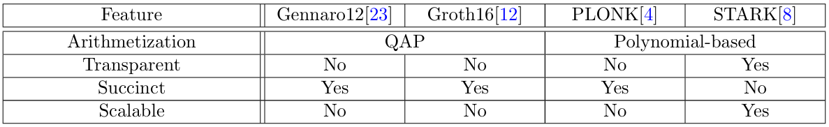
Table 12 compares the original SNARK protocol[23], Groth16[12] and PLONK[4], to the original STARK protocol[8] using the concepts introduced in this section. Section 3.2 explains the differences between PLONK[4], STARK[8], and their counterparts implemented by Plonky2.
Plonky2 implements variations of vanilla STARK and vanilla PLONK. In Starky, the correspondence between constraint and witness polynomials is evaluated globally as in vanilla PLONK, instead of locally as in vanilla STARK. Technically, this means polynomials representing this correspondence are defined in a way to evaluate to zero over the entire witness domain, instead of only where their respective constraints should hold. This is done using Lagrange polynomials as selector constraints. As a side-effect, Starky constraints become a mix of CPU and circuit representations, meaning one verbose constraint (receiving the entire current and next states as input) is selected per transition.
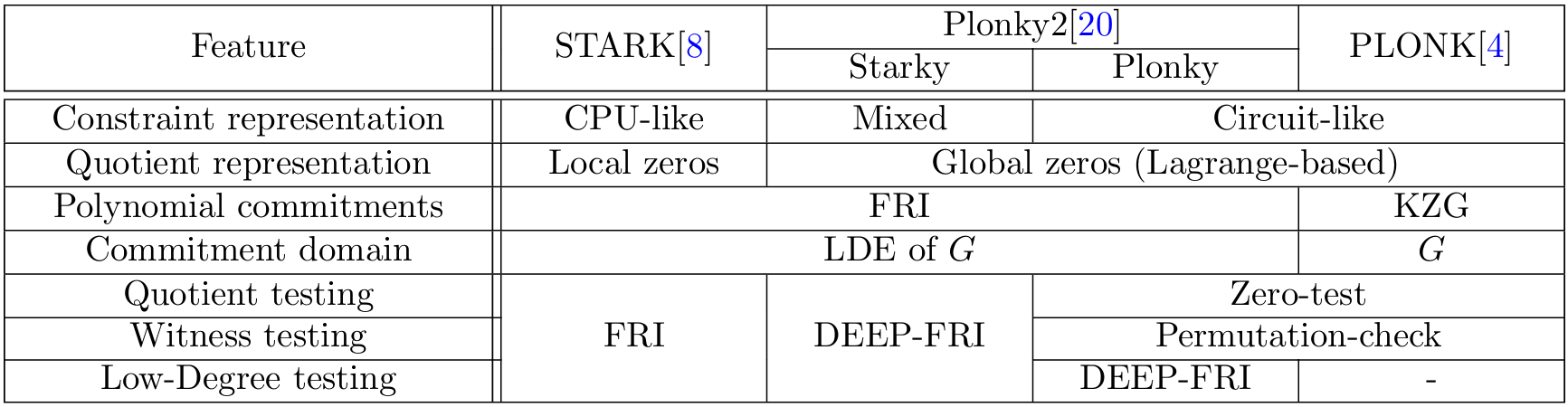
In Plonky, these correspondence polynomials are committed using DEEP-FRI[9] instead of KZG[2], the original commitment scheme used in vanilla PLONK, which removes the need for a CRS and makes Plonky transparent. As a side-effect, Plonky polynomials must be extended to a larger domain as required by DEEP-FRI. The rest of the polynomial evaluations are still required because the arithmetization process is maintained. Table 13 compares STARK, PLONK, Starky and Plonky.
An important detail about Plonky2 is the choice of Goldilocks as the base field for polynomial representation. This field is fully compatible with 32-bit architectures but requires some algebraic tricks to represent larger values. There are no native 64-bit operations in the MIPS version implemented by zkMIPS, but a similar trick is required to represent 32-bit GPRs as pairs of 16-bit columns. Even though 16-bit columns increase the space necessary to represent GPRs, it results in smaller proofs. This trade-off and other details about zkMIPS architecture will be explained in Section 4.
The first step to prove the correct execution of a MIPS program inside zkMIPS is to collect every internal CPU state during the program execution. This can be done on the Prover side by running the program and logging into a table the value of each CPU variable after each instruction execution. This table is a preliminary version of the trace record and contains the columns described in Table 2. This preliminary trace allows the direct verification of state transitions during program execution by checking whether each pair of subsequent rows matches the MIPS CPU state transition function.
The exact transition function implied by each instruction is defined according to the MIPS specifications (see Tables 4 to 10) and the way it is proved in a zkVM depends on the chosen proof model. In order to simplify the design of zkMIPS proving procedure and increase its efficiency, we decided to divide it in three dependent layers illustrated in Figure 2 and described below.
First layer: Continuation In this first layer the program execution is divided into small sequential executions called segments. Each segment is proved independently in the second proving layer. We call the trace from to this layer the program trace to distinguish from traces from other layers. It is important to stress that the program trace is not explicitly logged in practice; instead, the MIPS VM running on the first layer only logs the first and the last CPU states from each segment. When all proofs from the second layer have been produced, they are recursively combined into one single proof for the correct execution of the entire program trace. This process is called continuation and, for this reason, the proofs recursively produced in this layer are called continuation proofs.
Second layer: Segmentation In this intermediary layer each segment execution is divided into smaller, non-sequential, executions called modules, named in a reference to CPU modules responsible for special instructions processing. Each module combines all segment instructions from an independent subset of MIPS instructions and is proved independently in the third proving layer. Namely, the main proving modules are arithmetic, logic, memory and control, and the instructions proved by them are described in Table 14. In addition to these, a special Poseidon hashing module is simulated through modules optimized for this operation, namely the Poseidon and Poseidon-Sponge modules. We call the traces from to this layer segment traces to distinguish from traces from other layers. Unlike the program trace, segment traces must be logged. When all proofs from the third layer have been produced, a lookup scheme is used to prove their traces match the segment trace. At the end, this lookup proof and third layer proofs are combined into one single proof called the segment proof.
Third layer: Modularization In this final layer each module execution is proved independently using specialized STARK proofs. Traces proved in the third layer are called module traces and they do not contain repeated instructions, as might be the case for segment traces. This layer is where transition functions are finally proved, resulting in independent proofs called module proofs. We consider instructions repeated if they execute the same MIPS instruction with the same input values in the same order, but with possibly different input registers (only the values stored in these registers must be the same). This property can slightly prevent redundancy and improve performance.
It should be clear that continuation proofs cannot be produced in the first layer before segment proofs have been produced in the second layer because continuation proofs depend on segment proofs. On the other hand, segment proofs can in theory be produced in the second layer before module proofs have been produced because segment proofs are simply lookup proofs from segment to module traces (both types of traces are produced in the second layer). However, second and third layers usually run in sequence because there is little advantage in running them in parallel for practical segment sizes.
Parallelization can additionally be applied between different instances of the second layer. For large programs, many segment provers can work together in parallel to generate segment proofs faster, resulting huge performance gains in the second layer as all provers run roughly in the time of a single one. In this setup continuation provers can also run in parallel, making the continuation layer finish in time logarithmic to the number of segments (continuation provers depend on segment or other continuation proofs, as can be seen in Figure 1). This distributed proving system is known as Provers network.
The main and additional proving layers described in Figure 1 are the same described in Figure 2. The main proving layers and how their proofs are composed will be explained in Sections 4.1 to 4.3, while the additional layer and the choice of the proof system it uses will be described in Section 4.4.
The first proving layer in zkMIPS proves that segments are consistent with each other. This layer runs in two steps that are invoked separately by the entity proving the program. First, zkMIPS is invoked to run the input program and divide its execution into segments, which happens independently of the main proving procedure. When all segment proofs have been generated, this layer is invoked again to combine them into a single proof that shows the correctness of the entire program execution.
The program division procedure periodically pauses the VM running the MIPS program after a constant number of instructions (the size of segments, which is received as input by zkMIPS) and stores the memory state, the PC and the cycle counter for that moment. This set of variables is called the image id and it is given as public input to the segment prover as it tells exactly where and how to start the proving procedure. A compressed version of the image id is given as public input to the segment prover. This compression replaces the memory state with a Merkle tree of the memory state, which is enough for the Verifier to check memory access made by the Prover using Merkle paths.
When the continuation prover is invoked, image ids are used to show subsequent segments match, by comparing the initial image id of each segment with the last image id of the previous segment. Once the proof for the correspondence of a pair of subsequent segments is ready, their underlying polynomials and FRI proofs are batched together (segment proofs are Starky) and attached to their correspondent proof, resulting in a proof for the execution of the larger segment trace.
This procedure is repeated recursively until a single proof for the entire program trace is obtained. This is possible because the continuation is the same for segments of any size, independent of whether they were produced by segment or continuation provers. Because continuation proofs are mostly FRI proofs, whose verification steps are also recursive, a verifier circuit for these proofs is relatively simple. The continuation prover is written using Plonky instead of Starky, which reduces proof size, proving time and verification complexity. The fact that Plonky and Starky use the same field and have their polynomials low-degree tested by the same protocol makes them fully compatible and composable.
The second proving layer is where the most expressive parts of zkMIPS proofs are generated. Given memory state, PC and cycle counter from the beginning of a segment, this prover executes the program from that point and collect memory hashes from each instruction of that segment. The image id from the last instruction is the output of that proof and should be equal to the input of the next proof.
Segment and module traces are divided into columns containing 16-bit values. Because proofs are written using Plonky2, 16-bit values are represented by Goldilocks elements, which are 64-bit. A lookup verifies that values stored inside these columns are within a 16-bit range. This lookup uses a special range counter column containing all values allowed. The reason for this 64-bit representation of 16-bit values comes from a trade-off: 16-bit values imply 216 elements in the range counter column and a segment size at least this large; 32-bit values would make the segment size greater than 232. Empirically, segment sizes between 218 and 223 (which are compatible to 16-bit range checks but not with 32-bit range checks) result in the better performance than smaller or larger segment sizes.
Since MIPS is a 32-bit architecture, the values stored in GPRs take up two columns each. However, segment and module trace columns do not contain values from all GPRs in every cycle. Instead of logging GPRs directly into the main trace, the segment prover logs them into a register file in the format of Table 2, and then converts these values to a trace in the format of Table 15.
Including all registers in the main trace requires copy constraints to ensure values do not change when they do not have to (when a register is not touched during the execution of an instruction). Logging 32 register values of 32-bit each into 16-bit trace columns would require 64 columns for these values, and 32 columns for variables selecting their copy constraints. Currently, zkMIPS trace record has 57 columns, meaning GPR inclusion would increase trace size by more than 150%.
Each state of the register file where GPRs are logged to must be written to zkMIPS memory. This means memory needs to be accessed after each instruction and register consistency is guaranteed by memory and Poseidon modules (memory accesses require Poseidon-based Merkle paths) instead of the segment proof. This approach might seem costly at first, but it completely removes the need for copy constraints because the register file can be succinctly modified by constraint polynomials that change specific memory positions, e.g. those memory words storing individual GPRs.
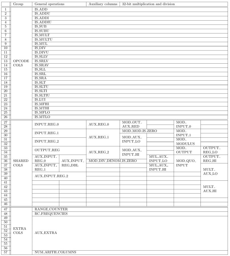
These 57 trace columns are divided into three main groups described below:
Once the segment and module traces have been generated, which happens in parallel as they encode the same rows, they are compiled into segment and module trace polynomials. In parallel to module proving, the segment prover can compile segment and module columns to LogUp polynomials.
The third proving layer is where the most meaningful parts of zkMIPS proofs are processed. This layer ensures the correctness of polynomials defined in segment proofs. In practice, there is no distinction between these proving layers; the distinction made in this document is conceptual and tries to abstract what is proved by pure Starky (third layer) from what is proved by lookup proofs (second layer).
Witness polynomials for segment and module proofs can be generated and processed in parallel because they are technically the same. Segment and module columns evaluate to the same values in the same order, with segment columns being defined sequentially and module columns non-sequentially; in other words, the set of values in segment columns equals the union of set of values in module columns. On the other hand, constraint polynomials for segment and module proofs are substantially different since segment proofs represent lookups.
After segment and module witness generation, module proofs are generated by their respective module provers, while segment proofs are generated by the LogUp prover. At this point, the order in which these proof are generated is irrelevant Once all of these proofs have been generated, they are batched into a final segment proof. The actual segment proof is, therefore, a combination of individual module proofs and the LogUp proof proving their correspondence to the segment trace.
The optional proving layer compiles the final hash-based continuation proof into an elliptic-curve-based Groth16 proof. The verification of this proof requires a pairing function that is natively supported by the EVM. This improves on-chain verification performance because the hash function used in FRI verification do not have to be simulated on-chain. Instead, only a succinct verification of this hash function is performed by means of a Groth16 proof for the hash function verification algorithm.
Given a hash of the initial memory state of a program, the final continuation proof guarantees there exists a sequence of valid CPU states that halts a MIPS VM at a valid result starting from the first instruction of that program. By design, this property ensures logic, memory and register integrity.
A lot of efficient zkVMs have appeared over the last months[22, 29, 27], changing the scenario and the perspective for applications based on this technology. These zkVMs can be categorized depending on their native EVM-compatible[30]. zkMIPS sits in the furthest EVM-compatible category, meaning it proves real-world programs instead of smart contracts. Still, zkMIPS proofs can be verified on chain and can verify Ethereum (or any other blockchain) statements through real-world programs that witness these statements given proper EVM data such as smart-contract data, block hashes, account address, etc.
EVM-compatibility can be achieved through native Golang and Rust support, allowing EVM simulators written in those languages to be proven once they are compiled to MIPS. The prioritization of support for these languages stems from the prevalence of these languages within blockchain development. Golang and Rust support is ensured by a careful selection of MIPS instructions that include opcodes used by these languages default compilers, go[10] and rustc[24]. Using minigeth[18] (a Golang based EVM verifier), zkMIPS can prove Ethereum transactions in 30 minutes on a 128-CPU server; the same task can be performed in less than one minute using REVM[5] (a Rust-based EVM verifier).
This 30x performance improvement from Golang to Rust-based verification is due to technical differences between these languages and their compilers, which results in significantly fewer instructions in a rustc-compiled program that executes the same functionality as the go-compiled one. This performance can be improved further for blocks with many transactions if a Prover network is used to generate segment proofs. When using a Prover network, one must also consider the cost of aggregating segment proofs, which takes 0.9 seconds on a 128-CPU server, and 0.6 seconds on a 64-core GPU.
If the proof must be verified on-chain, an additional Groth16 proof should be produced, which takes around 1.7 seconds on CPU machines and 0.8 seconds on GPU machines, and produces proofs of 414KB. As for the RAM consumption, zkMIPS requires at least 17GB when proving segments of size 214, and this number goes up to 27GB for segments of size 218, allowing Provers to run on desktops. In general, for a single Prover running on a 128-CPU server, zkMIPS achieves ∼8kHz (8k proved instructions per second); on a 64-core GPU, this performance increases to ∼13kHz.
